
Top Related Projects

Google's Operations Research tools:

A Python-embedded modeling language for convex optimization problems.

SciPy library main repository

An object-oriented algebraic modeling language in Python for structured optimization problems.

Modeling language for Mathematical Optimization (linear, mixed-integer, conic, semidefinite, nonlinear)
Quick Overview
PuLP is an open-source linear programming modeler written in Python. It allows users to describe optimization problems using Python objects and then solve these problems using a variety of solvers. PuLP is designed to be intuitive and easy to use, making it accessible for both beginners and experienced optimization practitioners.
Pros
- Easy to learn and use, with a Pythonic interface
- Supports multiple solvers, including open-source and commercial options
- Handles both linear and integer programming problems
- Actively maintained with good documentation and community support
Cons
- Performance may be slower compared to specialized commercial solvers
- Limited to linear and integer programming (no support for nonlinear optimization)
- Dependency on external solvers for solving problems
- May require additional setup for some solvers
Code Examples
- Creating a simple linear programming problem:
from pulp import *

# Create the model
model = LpProblem(name="maximize-production", sense=LpMaximize)

# Define variables
x = LpVariable(name="x", lowBound=0)
y = LpVariable(name="y", lowBound=0)

# Add constraints
model += (2 * x + y <= 100, "material_constraint")
model += (x + y <= 80, "labor_constraint")

# Set objective
model += 3 * x + 2 * y

# Solve the problem
model.solve()

# Print the results
print(f"Optimal solution: x = {x.value()}, y = {y.value()}")
print(f"Objective value: {model.objective.value()}")
- Solving a binary knapsack problem:
from pulp import *

# Define problem data
items = ["A", "B", "C", "D"]
values = {"A": 6, "B": 4, "C": 5, "D": 7}
weights = {"A": 3, "B": 2, "C": 4, "D": 5}
capacity = 10

# Create the model
model = LpProblem(name="knapsack-problem", sense=LpMaximize)

# Define variables
x = LpVariable.dicts("item", items, cat="Binary")

# Add constraint
model += lpSum(weights[i] * x[i] for i in items) <= capacity

# Set objective
model += lpSum(values[i] * x[i] for i in items)

# Solve the problem
model.solve()

# Print results
print("Selected items:")
for i in items:
    if x[i].value() == 1:
        print(f"- {i}")
print(f"Total value: {model.objective.value()}")
- Solving a transportation problem:
from pulp import *

# Define problem data
sources = ["A", "B"]
destinations = ["1", "2", "3"]
costs = {("A", "1"): 2, ("A", "2"): 3, ("A", "3"): 4,
         ("B", "1"): 3, ("B", "2"): 2, ("B", "3"): 1}
supply = {"A": 50, "B": 70}
demand = {"1": 30, "2": 40, "3": 50}

# Create the model
model = LpProblem(name="transportation-problem", sense=LpMinimize)

# Define variables
x = LpVariable.dicts("route", costs, lowBound=0)

# Add constraints
for s in sources:
    model += lpSum(x[s, d] for d in destinations) <= supply[s]
for d in destinations:
    model += lpSum(x[s, d] for s in sources) >= demand[d]

# Set objective
model += lpSum(costs[route] * x[route] for route in costs)

# Solve the problem
model.solve()

# Print results
print("Optimal routes:")
for route in costs:
    if x[route].value() > 0:
        print(f"{route}: {x[route].value()}")
print(f"Total cost
Competitor Comparisons
Google's Operations Research tools:
Pros of OR-Tools
- More comprehensive optimization toolkit with support for various problem types
- Better performance for large-scale optimization problems
- Extensive documentation and examples
Cons of OR-Tools
- Steeper learning curve due to its complexity
- Requires compilation and installation of C++ libraries
Code Comparison
PuLP example:
from pulp import *
x = LpVariable("x", 0, 3)
y = LpVariable("y", 0, 1)
prob = LpProblem("myProblem", LpMaximize)
prob += x + y <= 2
prob += -4*x + y
OR-Tools example:
from ortools.linear_solver import pywraplp
solver = pywraplp.Solver.CreateSolver('GLOP')
x = solver.NumVar(0, 3, 'x')
y = solver.NumVar(0, 1, 'y')
solver.Add(x + y <= 2)
solver.Maximize(-4 * x + y)
Both PuLP and OR-Tools are powerful optimization libraries, but they cater to different needs. PuLP is more user-friendly and easier to get started with, making it suitable for simpler optimization problems and educational purposes. OR-Tools, on the other hand, offers a wider range of optimization capabilities and better performance for complex problems, but comes with a steeper learning curve and more complex setup process.
A Python-embedded modeling language for convex optimization problems.
Pros of CVXPY
- More powerful and flexible, supporting a wider range of optimization problems
- Better suited for advanced mathematical modeling and research applications
- Integrates well with other scientific Python libraries like NumPy and SciPy
Cons of CVXPY
- Steeper learning curve, especially for beginners in optimization
- May be overkill for simpler linear programming problems
- Potentially slower execution for basic linear programming tasks
Code Comparison
PuLP example:
from pulp import *
x = LpVariable("x", lowBound=0)
y = LpVariable("y", lowBound=0)
prob = LpProblem("MyProblem", LpMaximize)
prob += x + y <= 5
prob += x + 2*y <= 6
prob += x + y
prob.solve()
CVXPY example:
import cvxpy as cp
x = cp.Variable()
y = cp.Variable()
constraints = [x >= 0, y >= 0, x + y <= 5, x + 2*y <= 6]
objective = cp.Maximize(x + y)
prob = cp.Problem(objective, constraints)
prob.solve()
Both PuLP and CVXPY are popular optimization libraries for Python, but they cater to different user needs and problem complexities. PuLP is generally easier to use for beginners and more efficient for simple linear programming problems, while CVXPY offers more advanced features and flexibility for complex optimization tasks.
SciPy library main repository
Pros of SciPy
- Broader scope, covering a wide range of scientific computing tasks
- More extensive documentation and community support
- Highly optimized and efficient implementations of numerical algorithms
Cons of SciPy
- Steeper learning curve due to its extensive functionality
- May be overkill for simple linear programming tasks
- Requires additional dependencies for certain functionalities
Code Comparison
PuLP example:
from pulp import *
prob = LpProblem("Simple LP Problem", LpMaximize)
x = LpVariable("x", lowBound=0)
y = LpVariable("y", lowBound=0)
prob += x + y <= 2
prob += -4*x + y
SciPy example:
from scipy.optimize import linprog
c = [-1, -1]
A = [[1, 1]]
b = [2]
res = linprog(c, A_ub=A, b_ub=b, method="simplex")
PuLP is more intuitive for linear programming problems, while SciPy's linprog function requires a different approach to problem formulation. SciPy offers a broader range of optimization methods but may be less straightforward for simple LP problems compared to PuLP's declarative style.
An object-oriented algebraic modeling language in Python for structured optimization problems.
Pros of Pyomo
- More extensive modeling capabilities, including support for nonlinear and discrete optimization
- Ability to handle larger and more complex problems
- Greater flexibility in model formulation and solver selection
Cons of Pyomo
- Steeper learning curve and more complex syntax
- Slower model construction for simpler problems
- Requires separate installation of solvers
Code Comparison
Pyomo example:
from pyomo.environ import *

model = ConcreteModel()
model.x = Var(domain=NonNegativeReals)
model.y = Var(domain=NonNegativeReals)
model.obj = Objective(expr=model.x + 2*model.y, sense=maximize)
model.con = Constraint(expr=3*model.x + 4*model.y <= 12)
PuLP example:
from pulp import *

prob = LpProblem("MyProblem", LpMaximize)
x = LpVariable("x", lowBound=0)
y = LpVariable("y", lowBound=0)
prob += x + 2*y
prob += 3*x + 4*y <= 12
Both Pyomo and PuLP are powerful optimization modeling tools, but they cater to different user needs. Pyomo offers more advanced features and flexibility, making it suitable for complex problems, while PuLP provides a simpler interface for straightforward linear programming tasks.
Modeling language for Mathematical Optimization (linear, mixed-integer, conic, semidefinite, nonlinear)
Pros of JuMP.jl
- Higher performance due to Julia's speed and JIT compilation
- More expressive modeling language with support for complex constraints
- Better integration with Julia's ecosystem for scientific computing
Cons of JuMP.jl
- Steeper learning curve, especially for those unfamiliar with Julia
- Smaller community and fewer resources compared to PuLP's Python ecosystem
- Less mature and potentially less stable than PuLP
Code Comparison
PuLP example:
from pulp import *
x = LpVariable("x", 0, 3)
y = LpVariable("y", 0, 1)
prob = LpProblem("myProblem", LpMinimize)
prob += x + y <= 2
prob += -4*x + y
JuMP.jl example:
using JuMP, GLPK
model = Model(GLPK.Optimizer)
@variable(model, 0 <= x <= 3)
@variable(model, 0 <= y <= 1)
@constraint(model, x + y <= 2)
@objective(model, Min, -4x + y)
Both PuLP and JuMP.jl are powerful optimization modeling languages, but they cater to different ecosystems and user preferences. PuLP is more accessible for Python users, while JuMP.jl offers higher performance and tighter integration with Julia's scientific computing capabilities.
Convert  designs to code with AI
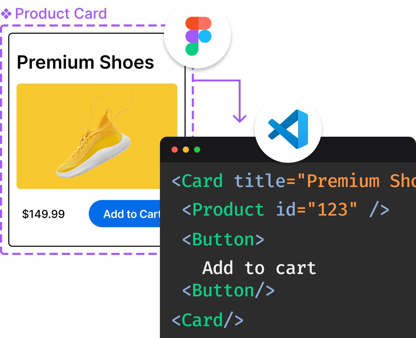
Introducing Visual Copilot: A new AI model to turn Figma designs to high quality code using your components.
Try Visual CopilotREADME
pulp
.. image:: https://travis-ci.org/coin-or/pulp.svg?branch=master :target: https://travis-ci.org/coin-or/pulp .. image:: https://img.shields.io/pypi/v/pulp :target: https://pypi.org/project/PuLP/ :alt: PyPI .. image:: https://img.shields.io/pypi/dm/pulp :target: https://pypi.org/project/PuLP/ :alt: PyPI - Downloads

PuLP is an linear and mixed integer programming modeler written in Python. With PuLP, it is simple to create MILP optimisation problems and solve them with the latest open-source (or proprietary) solvers. PuLP can generate MPS or LP files and call solvers such as GLPK_, COIN-OR CLP/CBC, CPLEX, GUROBI_, MOSEK_, XPRESS_, CHOCO_, MIPCL_, HiGHS_, SCIP_/FSCIP_, and OR-Tools CP-SAT_ (via the CPSAT API).
The documentation for PuLP can be found here <https://coin-or.github.io/pulp/>_.
PuLP is part of the COIN-OR project <https://www.coin-or.org/>_.
.. important::
CBC is not shipped inside the PuLP package. Older releases bundled a CBC
binary and exposed it as PULP_CBC_CMD; that API and the bundled solver are
removed. To solve models with CBC through PuLP you should:
- install PuLP with the optional CBC extra:
python -m pip install pulp[cbc](this installs thecbcbox <https://pypi.org/project/cbcbox/>_ wheel, which provides a CBC executable PuLP can find automatically), or - install a CBC build yourself and ensure the
cbc(orcbc.exeon Windows) executable is on yourPATH,
then use the COIN_CMD solver (or call prob.solve() with no arguments
when CBC is available; otherwise install another solver such as GLPK or pass
an explicit solver). Without CBC or another available solver, the default
solve path will raise PulpError: No solver available.
Installation
PuLP requires Python 3.10 or newer.
Recommended: install with CBC support::
python -m pip install pulp[cbc]
Plain python -m pip install pulp installs only the modeler; you must then
supply your own CBC on PATH or another solver.
Otherwise follow the download instructions on the PyPi page <https://pypi.python.org/pypi/PuLP>_.
Installing solvers
PuLP can use a variety of solvers. When CBC is available (via pulp[cbc] or
cbc on PATH), COIN_CMD is the usual open-source MIP/LP choice and is
selected as the default ahead of GLPK. PuLP can also install other solvers via
optional PyPI extras (some require a commercial license for running or for large models)::
python -m pip install pulp[gurobi]
python -m pip install pulp[cplex]
python -m pip install pulp[xpress]
python -m pip install pulp[scip]
python -m pip install pulp[highs]
python -m pip install pulp[copt]
python -m pip install pulp[mosek]
python -m pip install pulp[ortools]
python -m pip install pulp[cylp]
python -m pip install pulp[cbc]
If you want to install all open source solvers (scip, highs, cbc), you can use the shortcut:: python -m pip install pulp[open_py]
For more information on how to install solvers, see the guide on configuring solvers <https://coin-or.github.io/pulp/guides/how_to_configure_solvers.html>_.
Quickstart
Use LpProblem to create a problem, then add variables with add_variable. Create a problem called "myProblem" and a variable x with 0 ⤠x ⤠3::
 from pulp import *
 prob = LpProblem("myProblem", LpMinimize)
 x = prob.add_variable("x", 0, 3)
To create a binary variable y (values 0 or 1)::
y = prob.add_variable("y", cat="Binary")
Combine variables to create expressions and constraints and add them to the problem::
prob += x + y <= 2
An expression is a constraint without a right-hand side (RHS) sense (one of =, <= or >=). If you add an expression to a problem, it will become the objective::
prob += -4*x + y
To solve the problem with the default solver (CBC when installed via pulp[cbc]
or cbc on PATH, otherwise another available backend)::
status = prob.solve()
If you want to try another solver to solve the problem::
status = prob.solve(GLPK(msg = 0))
To use the OR-Tools CP-SAT solver (install with python -m pip install pulp[ortools]).
Every variable must have finite lower and upper bounds; continuous variables are
solved on their integer-rounded domain::
 from pulp import CPSAT
 status = prob.solve(CPSAT(msg=False))
Display the status of the solution::
 LpStatus[status]
 > 'Optimal'
You can get the value of the variables using value. ex::
 value(x)
 > 2.0
Essential Classes
These types form the usual modelling workflow: create an LpProblem, attach
LpVariable instances with add_variable, build linear expressions (often
with lpSum / lpDot / lpSum_vars / lpSum_vars_coefs), combine them
into LpConstraint rows, and call solve.
-
LpProblem-- Container for an LP or MIP: variables, objective, constraints, and solve API -
LpVariable-- A decision variable belonging to one problem; used inside expressions and constraints -
LpAffineExpression-- A linear combination of variables and a constant (objectives, constraint bodies, intermediate terms) -
LpConstraint-- A single row relating an affine expression to a bound with<=,=, or>=:a1x1 + a2x2 + ... + anxn (<=, =, >=) b
Useful Functions
value()-- Finds the value of a variable or expressionlpSum()-- Given a list of the form [a1x1, a2x2, ..., an*xn] will construct a linear expression to be used as a constraint or variablelpDot()-- Given two lists of the form [a1, a2, ..., an] and [x1, x2, ..., xn] will construct a linear expression to be used as a constraint or variablelpSum_vars()-- Sum of variables with coefficient 1 each (batch construction)lpSum_vars_coefs()-- Sum ofcoeff * varpairs from an iterable of(variable, coefficient)(batch construction)
More Examples
Several tutorial are given in documentation <https://coin-or.github.io/pulp/CaseStudies/index.html>_ and pure code examples are available in examples/ directory <https://github.com/coin-or/pulp/tree/master/examples>_ .
The examples assume CBC is available (for example after pip install pulp[cbc]).
To use other solvers they must be available (installed and accessible). For more
information, see the guide on configuring solvers <https://coin-or.github.io/pulp/guides/how_to_configure_solvers.html>_.
For Developers
If you want to install the latest version from GitHub you can run::
python -m pip install -U "pulp[cbc] @ git+https://github.com/coin-or/pulp.git"
Building from source
This version of PuLP includes a Rust extension (pulp._rustcore) that provides the core model, variables, constraints, and expressions. The build uses maturin <https://github.com/PyO3/maturin>_ and requires a Rust toolchain in addition to Python.
Requirements
- Python 3.10 or newer
- Rust (latest stable). Install from https://rustup.rs/
- uv (recommended for install and dev). See the
uv documentation <https://docs.astral.sh/uv/>_ for installation. - OS: Windows, macOS (x86_64, arm64), or Linux (x86_64, arm64). The Rust extension is built for the host platform.
Build steps
From the PuLP root directory, create a virtual environment and install the package in editable mode with dev dependencies::
uv venv
uv pip install --group dev -e .[cbc]
Or with plain pip (maturin will be used automatically by the build backend)::
python -m venv .venv
source .venv/bin/activate   # Windows: .venv\Scripts\activate
python -m pip install --upgrade pip
python -m pip install -e ".[cbc]"
Running tests
::
uv run python -m unittest discover -s pulp/tests -v
Building the documentation
The PuLP documentation is built with Sphinx <https://www.sphinx-doc.org>_. Use a virtual environment and the dev install above, then::
cd doc
make html
A folder named html will be created inside doc/build/. Open doc/build/html/index.html in a browser.
Contributing to PuLP
Instructions for making your first contribution to PuLP are given here <https://coin-or.github.io/pulp/develop/contribute.html>_.
Comments, bug reports, patches and suggestions are very welcome!
- Comments and suggestions: https://github.com/coin-or/pulp/discussions
PuLP Google Group <https://groups.google.com/g/pulp-or-discuss>_ â community discussion and Q&A- Bug reports: https://github.com/coin-or/pulp/issues
- Patches: https://github.com/coin-or/pulp/pulls
Copyright and License
PuLP is distributed under an MIT license.
 Copyright J.S. Roy, 2003-2005
 Copyright Stuart A. Mitchell
 See the LICENSE file for copyright information.
.. _Python: http://www.python.org/
.. _GLPK: http://www.gnu.org/software/glpk/glpk.html .. _CBC: https://github.com/coin-or/Cbc .. _CPLEX: http://www.cplex.com/ .. _GUROBI: http://www.gurobi.com/ .. _MOSEK: https://www.mosek.com/ .. _XPRESS: https://www.fico.com/es/products/fico-xpress-solver .. _CHOCO: https://choco-solver.org/ .. _MIPCL: http://mipcl-cpp.appspot.com/ .. _SCIP: https://www.scipopt.org/ .. _HiGHS: https://highs.dev .. _FSCIP: https://ug.zib.de .. _CP-SAT: https://developers.google.com/optimization/cp/cp_solver
Top Related Projects
Google's Operations Research tools:
A Python-embedded modeling language for convex optimization problems.
SciPy library main repository
An object-oriented algebraic modeling language in Python for structured optimization problems.
Modeling language for Mathematical Optimization (linear, mixed-integer, conic, semidefinite, nonlinear)
Convert designs to code with AI
Introducing Visual Copilot: A new AI model to turn Figma designs to high quality code using your components.
Try Visual Copilot